5 R Programming Language
Iddawela
In 1996, two academics from the University of Auckland, New Zealand, launched a new programming language.
25 years later, this language is one of the most widely used in the world.
Here’s the story of R:
Iddawela (2023) Twitter Thread
5.1 Reinsurance
Policy Tensor
Reinsurers are basically giant pools of capital that agree to absorb catastrophe losses from the insurers in exchange for ceded premium. This allows the insurers to compete for market share without worrying too much about the buildup of risks on their balance sheets. This is what allows you to buy insurance on your house or car cheaply, quickly, and rather effortlessly.
The crucial assumption that allows reinsurance to work is that insured catastrophes are “acts of god” that are basically uncorrelated. So, in any given year, you might have to shell out money for a hurricane here, a flooding there, a wildfire somewhere else. This is a profitable business only as long as the joint probability of all risks for which you’re on the hook is roughly the product of the probability of individual catastrophes—and the product of small fractions is a very small fraction indeed. This crucial assumption is now breaking down.
The present conjuncture features, “an inflation shock that emanates from the disruptions caused by a pandemic, the policy responses to that pandemic and an energy shock caused by a war,” a war that is itself due to “the breakdown in relations among great powers”; a crisis of global macroeconomic stability due to the sudden revival of hard-currency monetary cycles to fight said inflation; a crisis of “political stability in many high-income democracies”; and, supervising this ensemble of crises, the meta-crisis of global heating. These crises are irreducibly codependent. This “polycrisis as a social scientific wake-up call,” says simply, “LOOK at the interaction term!” The climate crisis is the meta-crisis that undergirds the polycrisis.
Fitch Ratings, and other industry sources, are expecting “a dramatic tightening in the market”. Why? Because the losses are mounting.
The rapidly rising frequency, amplitude and correlation of “natural” catastrophes due to global heating poses an existential risk to the industry. No one knows how long the industry can survive — it is completely exposed to the risk that we will fail to temper global heating.
It’s not for some random reasons we are now, at this time, in a world where the interaction term has acquired particular force. The reasonably stable world is gone for reasons endogenous to modernity. Specifically, the assassin is Ulrich Beck. Beck spelled out the multiple ways in which risk is manufactured at scale by industrial modernity.
Writing in the aftermath of Chernobyl, Beck described the transition to a very different kind of world; one where the sacred violence of the gods is replaced by the blind violence of the big machine of industrial modernity. Existential risks to our civilization are now all anthropogenic: nuclear war, global heating, anthropogenic pandemics, super AI, etc.
The issue is that we’re riding a hockey stick of capabilities that is simultaneously a constantly accelerating source of risk production in the sense identified by Beck. What we need, in order to be self-aware historical actors in the polycrisis, is a sense of exponential time. As we ride up the hockey-stick, the weight of our species on the web of life increases exponentially; in effect, accelerating the passage of time. To put it somewhat tongue-in-cheek, a 2% growth rate means bigger and bigger absolute additions to the familiar pie, which, recall, doubles up as catastrophic risk exposure in the Beckian frame.
5.2 Superspreaders
Wong
Superspreading has been recognized as an important phenomenon arising from heterogeneity in individual disease transmission patterns (1). The role of superspreading as a significant source of disease transmission has been appreciated in outbreaks of measles, influenza, rubella, smallpox, Ebola, monkeypox, SARS, and SARS-CoV-2 (1, 2). A basic definition of an nth-percentile superspreading event (SSE) has been proposed to be any infected individual who infects more people than does the nth-percentile of other infected individuals (1). Hence, if the number of secondary cases is randomly distributed, then for large n, SSEs can be viewed as right-tail events. A natural language for understanding the tail events of random distributions is extreme value theory, which has been applied to contexts as diverse as insurance (3) and contagious diseases (4). Here, we apply extreme value theory to empirical data on superspreading in order to gain insight into this critical phenomenon impacting the current COVID-19 pandemic.
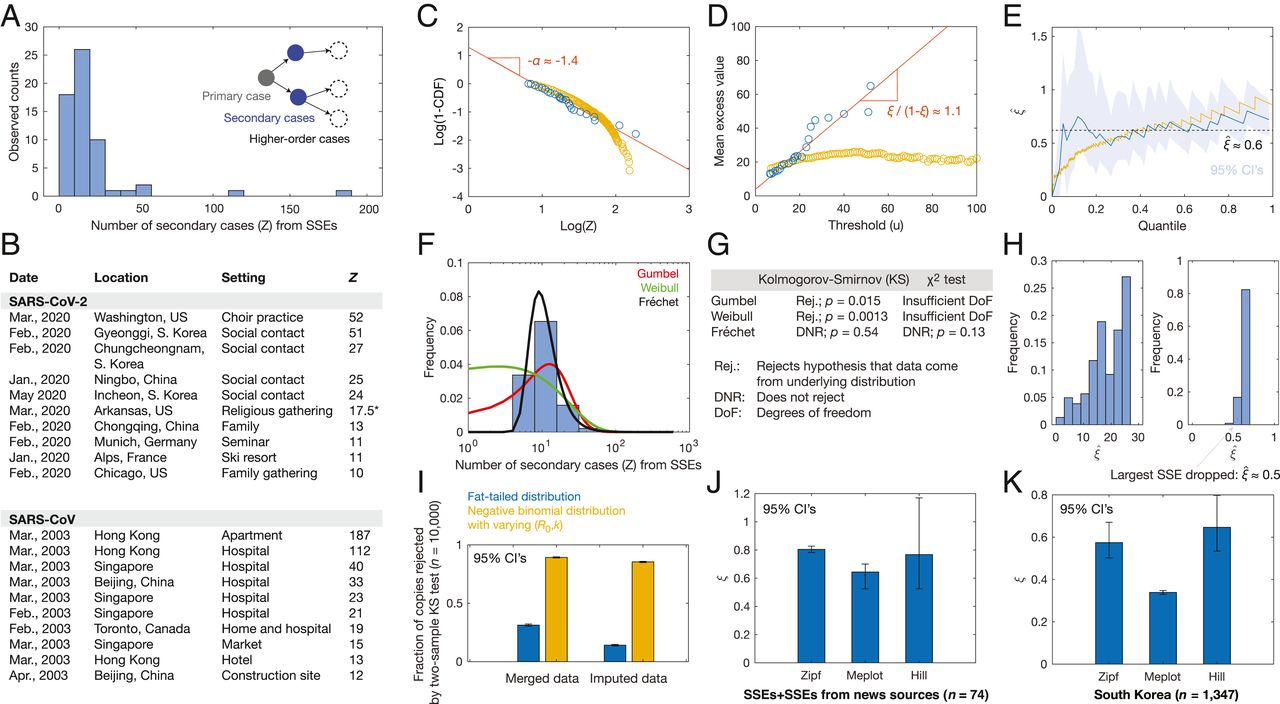
Figure: SARS-CoV and SARS-CoV-2 SSEs correspond to fat tails. (A) Histogram of Z for 60 SSEs. (B) Subsample of 20 diverse SARS-CoV and SARS-CoV-2 SSEs. *See Dataset S1 for details. (C) Zipf plots of SSEs (blue) and 10,000 samples of a negative binomial distribution with parameters (R0,k) = (3,0.1), conditioned on Z > 6 (yellow). (D) Meplots corresponding to C. (E) Plots of \(\hat{ξ}\), the Hill estimator for ξ, for the samples in C. (F) Different extreme value distribution fits to the distribution of SSEs. (G) One-sample Kolmogorov–Smirnov and \(χ^{2}\) goodness-of-fit test results for the fits in F. (H) Robustness of results, accounting for noise (Left) and incomplete data (Right). (I) Inconsistency of the maxima of 10,000 samples of a negative binomial distribution (yellow) with the SSEs in A, accounting for variability in (R0,k) and data merging and imputation, in contrast to the maxima of 30 samples from a fat-tailed (Fréchet) distribution (blue) with tail parameter α = 1.7 and mean R0 = 3. The numbers of samples in each case were determined so that the sample mean of maxima is equal to the sample mean from A. (J–K) Generality of inferred \(ξ\) to 14 additional SSEs from news sources (J) and a dataset of 1,347 secondary cases arising from 5,165 primary cases in South Korea (K).
The Zipf plot shown in Fig.1C is a log-log plot of the survival function against the number of secondary cases, and the linearly decreasing behavior it shows suggests a power-law scaling of the form $Pr(Z>t)~t^{α} for large t. The value of the power-law coefficient, \(α≈1.45\) (95% CI: [1.38,1.51]), is greater than 1. Equivalently, this observation indicates that the tails of \(Z\) —as quantified by the threshold exceedance values \({Z_{i–u} | Z_{i} ≥u}\) —can be described by the generalized Pareto distribution, withcorresponding tail index \(ξ=1/α ≈ 0.7\) (95% CI: [0.62,0.76]). That \(ξ≤1\) is significant, since all moments higher than \(1/ξ\) diverge for a generalized Pareto distribution. The Zipf plot can be complemented by computing the mean excess function of \(Z\), \(e(u) = E(Z–u | Z≥u)\), which for a generalized Pareto distribution is linear in \(u\) with slope \(ξ/(1–ξ)\). Hence, checking for linearity in a plot of \(u\) against \(e(u) — a\) mean excess plot — above some threshold u allows one to verify the existence of fat tails. We observed in a meplot that for u>10, e(u) indeed increases approximately linearly with a slope of ~1.11 (Fig.1D; 95% CI: [1.02,1.20]; adjusted \(R^{2}\) : 0.91), suggesting a value of \(ξ≈0.5\), which is qualitatively consistent with the Zipf plot of Fig.1C
The Hill estimator of the tail index \(ξ\) is
\[\hat{ξ}(k) = \frac{1}{k} \sum_{i=1}^{k} log \frac{Z_{i,n}}{Z_{k,n}}\]
where 2≤k≤n and Z n,n ≤Z n-1,n ≤…≤Z 1,n are order statistics of the sample {Z i }. Plotting \(ξ\) against \(k\), we find that the value of \(ξ ≈0.6\) (95% CI: [0.4,1.0]) observed for a broad range of \(k\) is similar to the estimates above (Fig.1E). We found similar values of \(ξ\) for two other estimators, the Pickands and Dekkers-Einmahl-de Haan estimators. A negative binomial distribution of Z, with its exponential tail, would have predicted the distribution of SSEs to be Gumbel-like if each SSE were indeed a maximum of samples of \(Z\). This assertion can be proven by verifying the conditions
\[\underset{n\to \infty}{\lim} \frac{\sum_{n}^{\infty} P_{j}}{\sum_{n+1}^{\infty} P_{j}} = const\]
\[\underset{n\to \infty}{\lim} \sum_{n+2}^{\infty} \frac{P_{j}}{P_{n+1}}-\sum_{n+1}^{\infty}\frac{P_{j}}{P_{n}}= 0\]
where \(P_{j} =Pr(Z=j)\), sufficient for any discrete distribution to lie in a Gumbel-like domain of attraction. These considerations provide additional evidence suggesting that Z is not negative binomial.
Wong (2021) Coronavirus superspreading is fat-tailed (PNAS) (pdf) (pdf SM)
5.3 Vaccine
Madhi
A multicenter, double-blind, randomized, controlled trial to assess the safety and efficacy of the ChAdOx1 nCoV-19 vaccine (AZD1222) in people not infected with the human immunodeficiency virus (HIV) in South Africa. Participants 18 to less than 65 years of age were assigned in a 1:1 ratio to receive two doses of vaccine containing 5×10¹⁰ viral particles or placebo (0.9% sodium chloride solution) 21 to 35 days apart. Serum samples obtained from 25 participants after the second dose were tested by pseudovirus and live-virus neutralization assays against the original D614G virus and the B.1.351 variant. The primary end points were safety and efficacy of the vaccine against laboratory-confirmed symptomatic coronavirus 2019 illness (Covid-19) more than 14 days after the second dose.
Between June 24 and November 9, 2020, we enrolled 2026 HIV-negative adults (median age, 30 years); 1010 and 1011 participants received at least one dose of placebo or vaccine, respectively. Both the pseudovirus and the live-virus neutralization assays showed greater resistance to the B.1.351 variant in serum samples obtained from vaccine recipients than in samples from placebo recipients. In the primary end-point analysis, mild-to-moderate Covid-19 developed in 23 of 717 placebo recipients (3.2%) and in 19 of 750 vaccine recipients (2.5%), for an efficacy of 21.9% (95% confidence interval [CI], −49.9 to 59.8). Among the 42 participants with Covid-19, 39 cases (92.9%) were caused by the B.1.351 variant; vaccine efficacy against this variant, analyzed as a secondary end point, was 10.4% (95% CI, −76.8 to 54.8). The incidence of serious adverse events was balanced between the vaccine and placebo groups.
The primary efficacy analysis was end-point–driven for the composite of mild, moderate, or severe Covid-19 and required 42 cases to detect a vaccine efficacy of at least 60% (with a lower bound of 0% for the 95% confidence interval), with 80% power. Vaccine efficacy was calculated as 1 minus the relative risk, and 95% confidence intervals calculated with the Clopper–Pearson exact method are reported. Only participants in the per-protocol population (all participants who received two doses of vaccine or placebo and were grouped according to the injection they received, regardless of their planned group assignment) who were seronegative for SARS-CoV-2 at enrollment were included in the primary efficacy analysis. A sensitivity analysis was conducted that included seronegative participants in the modified intention-to-treat population (all participants who received two doses and were grouped by their planned assignment, irrespective of the injection they received). Confidence intervals reported in this article have not been adjusted for multiple comparisons.
Conclusions
A two-dose regimen of the ChAdOx1 nCoV-19 vaccine did not show protection against mild-to-moderate Covid-19 due to the B.1.351 variant.