3 Big Data Paradox
Bradley Abstract
Surveys are a crucial tool for understanding public opinion and behaviour, and their accuracy depends on maintaining statistical representativeness of their target populations by minimizing biases from all sources. Increasing data size shrinks confidence intervals but magnifies the effect of survey bias: an instance of the Big Data Paradox1. Here we demonstrate this paradox in estimates of first-dose COVID-19 vaccine uptake in US adults from 9 January to 19 May 2021 from two large surveys: Delphi–Facebook2,3 (about 250,000 responses per week) and Census Household Pulse4 (about 75,000 every two weeks). In May 2021, Delphi–Facebook overestimated uptake by 17 percentage points (14–20 percentage points with 5% benchmark imprecision) and Census Household Pulse by 14 (11–17 percentage points with 5% benchmark imprecision), compared to a retroactively updated benchmark the Centers for Disease Control and Prevention published on 26 May 2021. Moreover, their large sample sizes led to miniscule margins of error on the incorrect estimates. By contrast, an Axios–Ipsos online panel5 with about 1,000 responses per week following survey research best practices6 provided reliable estimates and uncertainty quantification. We decompose observed error using a recent analytic framework1 to explain the inaccuracy in the three surveys. We then analyse the implications for vaccine hesitancy and willingness. We show how a survey of 250,000 respondents can produce an estimate of the population mean that is no more accurate than an estimate from a simple random sample of size 10. Our central message is that data quality matters more than data quantity, and that compensating the former with the latter is a mathematically provable losing proposition.
Bradley (2021) Unrepresentative big surveys significantly overestimated US vaccine uptake
3.1 Quarantine fatigue thins fat-tailed impacts
Abstract Conte:
Fat-tailed damages across disease outbreaks limit the ability to learn and prepare for future outbreaks, as the central limit theorem slows down and fails to hold with infinite moments.
We demonstrate the emergence and persistence of fat tails in contacts across the U.S. We then demonstrate an interaction between these contact rate distributions and community-specific disease dynamics to create fat-tailed distributions of COVID-19 impacts (proxied by weekly cumulative cases and deaths) during the exact time when attempts at suppression were most intense.
Our stochastic SIR model implies the effective reproductive number also follows a fat-tailed stochastic process and leads to multiple waves of cases with unpredictable timing and magnitude instead of a single noisy wave of cases found in many compartmental models that introduce stochasticity via an additively-separable error term.
Public health policies developed based on experiences during these months could be viewed as an overreaction if these impacts were mistakenly perceived as thin tailed, possibly contributing to reduced compliance, regulation, and the quarantine fatigue.
While fat-tailed contact rates associated with superspreaders increase transmission and case numbers, they also suggest a potential benefit: targeted policy interventions are more effective than they would be with thin-tailed contacts.
If policy makers have access to the necessary information and a mandate to act decisively, they might take advantage of fat-tailed contacts to prevent inaction that normalizes case and death counts that would seem extreme early in the outbreak.
Our place-based estimates of contacts aid in these efforts by showing the dynamic nature of movement through communities as the outbreak progresses, which is quite costly to achieve in network models, forcing the assumption of static contact networks in many models.
In extreme value theory, fat tails confound efforts to prepare for future extreme events like natural disasters and violent conflicts because experience does not provide reliable information about future tail draws. However, impacts of extreme events play out over time based on policy and behavioral responses to the event, which are themselves dynamically informed by past experiences.
A general pattern of fat-tailed contact rate distributions across the U.S. suggests that fat tails in U.S. cases observed early in the outbreak are due to city- and county-specific contact networks and epidemiological dynamics.
By unpacking the dynamics that lead to the impacts of extreme events, we show that 1) fat-tailed impacts can also confound efforts to control and manage impacts in the midst of extreme events and 2) thin tails in disease impacts are not necessarily desirable, if they indicate an inevitable catastrophe.
Conte (2021) Quarantine fatigue thins fat-tailed coronavirus impacts (pdf) (pdf - SM)
3.2 Herd Immunity impossible with new Mutants
Professor of vaccinology Shabir Madhi at the University of the Witwatersrand says protecting at-risk individuals against severe Covid is more important than herd immunity
Leading vaccine scientists are calling for a rethink of the goals of vaccination programmes, saying that herd immunity through vaccination is unlikely to be possible because of the emergence of variants like that in South Africa.
The comments came as the University of Oxford and AstraZeneca acknowledged that their vaccine will not protect people against mild to moderate Covid illness caused by the South African variant.
Novavax and Janssen, which were trialled there in recent months and were found to have much reduced protection against the variant – at about 60%. Pfizer/BioNTech and Moderna have also said the variant affects the efficacy of their vaccines, although on the basis of lab studies only.
These findings recalibrate thinking about how to approach the pandemic virus and shift the focus from the goal of herd immunity against transmission to the protection of all at-risk individuals in the population against severe disease.
We probably need to switch to protecting the vulnerable, with the best vaccines we have which, although they don’t stop infection, they probably do stop you dying.
3.3 Danish Mask Study
Every study needs its own statistical tools, adapted to the specific problem, which is why it is a good practice to require that statisticians come from mathematical probability rather than some software-cookbook school. When one uses canned software statistics adapted to regular medicine (say, cardiology), one is bound to make severe mistakes when it comes to epidemiological problems in the tails or ones where there is a measurement error. The authors of the study discussed below (The Danish Mask Study) both missed the effect of false positive noise on sample size and a central statistical signal from a divergence in PCR results. A correct computation of the odds ratio shows a massive risk reduction coming from masks.
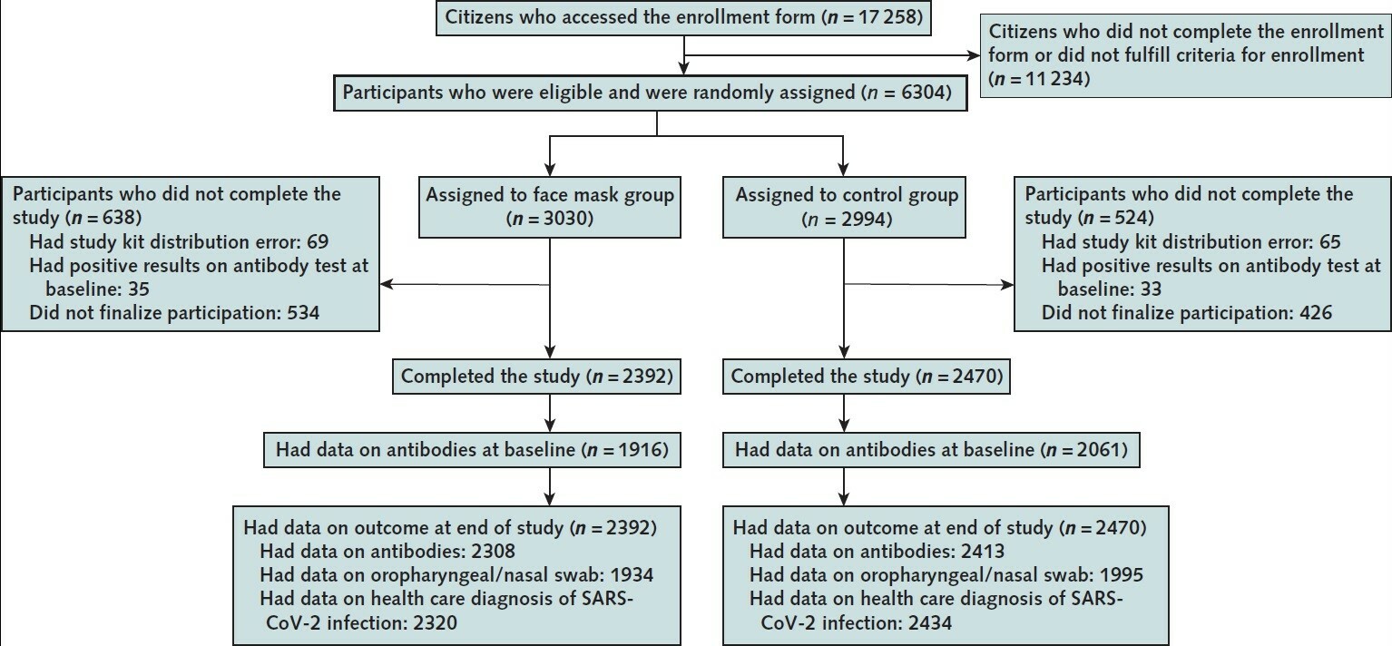
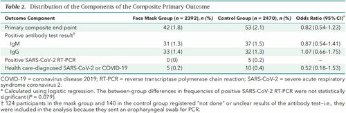
The article by Bundgaard et al., [“Effectiveness of Adding a Mask Recommendation to Other Public Health Measures to Prevent SARS-CoV-2 Infection in Danish Mask Wearers”, Annals of Internal Medicine (henceforth the “Danish Mask Study”)] relies on the standard methods of randomized control trials to establish the difference between the rate of infections of people wearing masks outside the house v.s. those who don’t (the control group), everything else maintained constant. The authors claimed that they calibrated their sample size to compute a p-value (alas) off a base rate of 2% infection in the general population. The result is a small difference in the rate of infection in favor of masks (2.1% vs 1.8%, or 42/2392 vs. 53/2470), deemed by the authors as not sufficient to warrant a conclusion about the effectiveness of masks.
…
Taleb’s Points:
The Mask Group has 0/2392 PCR infections vs 5/2470 for the Control Group. Note that this is the only robust result and the authors did not test to see how nonrandom that can be. They missed on the strongest statistical signal. (One may also see 5 infections vs. 15 if, in addition, one accounts for clinically detected infections.)
The rest, 42/2392 vs. 53/2470, are from antibody tests with a high error rate which need to be incorporated via propagation of uncertainty-style methods on the statistical significance of the results. Intuitively a false positive rate with an expected “true value” \(p\) is a random variable \(\rightarrow\) Binomial Distribution with STD \(\sqrt{n p (1-p)}\)
False positives must be deducted in the computation of the odds ratio.
The central problem is that both p and the incidence of infection are in the tails!
As most infections happen at home, the study does not inform on masks in general –it uses wrong denominators for the computation of odds ratios (mixes conditional and unconditional risk). Worse, the study is not even applicable to derive information on masks vs. no masks outside the house since during most of the study (April 3 to May 20, 2020), “cafés and restaurants were closed “, conditions too specific and during which the infection rates are severely reduced –tells us nothing about changes in indoor activity. (The study ended June 2, 2020). A study is supposed to isolate a source of risk; such source must be general to periods outside the study (unlike cardiology with unconditional effects).
The study does not take into account the fact that masks might protect others. Clearly this is not cardiology but an interactive system.
Statistical signals compound. One needs to input the entire shebang, not simple individual tests to assess the joint probability of an effect.
Comment from Tom Wenseleers For the 5 vs 0 PCR positive result the p value you calculate is flawed. The correct way to do it would e.g. be using a Firth logistic regression. Using R that would give you:
library(brglm)
summary(brglm(cbind(pcrpos, pcrneg) ~ treatment, family=binomial, data=data.frame(treatment=factor(c(“masks”,”nomasks”)),
pcrpos=c(0,5), pcrneg=c(2392,2470-5))))

2-sided p=0.11.
So that’s not significantly different.

Alternatively, you might use a Fisher’s exact test, which would give you :

fisher.test(cbind(c(0,2392),c(5,2470-5))):

2-sided p = 0.06.
Again, not significantly different.
A Firth logistic regression would be more appropriate though, since we have a clear outcome variable here and we don’t just want to test for an association in a 2×2 contingency table, as one would do using a Fisher’s exact test. For details see Firth, D. (1993). Bias reduction of maximum likelihood estimates. Biometrika 80, 27–38. A regular logistic regression doesn’t work here btw because of complete separation, https://en.wikipedia.org/wiki/Separation_(statistics) https://stats.stackexchange.com/questions/11109/how-to-deal-with-perfect-separation-in-logistic-regression. Going Bayesian would also be a solution, e.g. using the bayesglm() or brms package, or one could use an L1 or L2 norm or elastic net penalized binomial GLM model, e.g. using glmnet.
But the p value you calculate above is definitely not correct. Sometimes it helps to not try to reinvent the wheel.
The derivation of Fisher’s exact test you can find in most Statistics 101 courses, see e.g. https://mathworld.wolfram.com/FishersExactTest.html. For Firth’s penalized logistic regression, see https://medium.com/datadriveninvestor/firths-logistic-regression-classification-with-datasets-that-are-small-imbalanced-or-separated-49d7782a13f1 for a derivation. Or in Firth’s original article: https://www.jstor.org/stable/2336755?seq=1#metadata_info_tab_contents.
Technically, the problem with the way you calculated your p value above is that you use a one-sample binomial test, and assume there is no sampling uncertainty on the p=5/2470. Which is obviously not correct. So you need a two-sample binomial test instead, which you could get via a logistic regression. But since you have complete separation you then can’t use a standard binomial GLM, and have to use e.g. a Firth penalized logistic regression instead. Anyway, the details are in the links above.
You write “The probability of having 0 realizations in 2392 if the mean is \(\frac{5}{2470}\) is 0.0078518, that is 1 in 127. We can reexpress it in p values, which would be <.01”. This statement is obviously not correct then.
And if you didn’t do p values – well, then your piece above is a little weak as a reply on how the authors should have done their hypothesis testing in a proper way, don’t you think? If the 0 vs 5 PCR positive result is not statistically significant I don’t see how you can make a sweeping statement like “The Mask Group has 0/2392 PCR infections vs 5/2470 for the Control Group. Note that this is the only robust result and the authors did not test to see how nonrandom that can be. They missed on the strongest statistical signal.”. That “strong statistical signal” you mention turns out not be statistically significant at the p<0.05 level if you do your stats properly…
Taleb:You are conflating p values and statistical significance. Besides, I don’t do P values. https://arxiv.org/pdf/1603.07532.pdf
you can also work with Bayes Factors if you like. Anything more formal than what you have above should do really… But just working with a PMF of a binomial distribution, and ignoring the sampling error on the 5/2470 control group is not OK. And if you’re worried about the accuracy of p values you could always still calculate 95% confidence limits on them, right? Also not really what people would typically consider p-hacking…
Your title may a bit of a misnomer then. And as I mentioned: if one is worried about the accuracy of your p values & stochasticity on its estimated value, you can always calculate p-value prediction intervals, https://royalsocietypublishing.org/doi/10.1098/rsbl.2019.0174.
You are still ignoring the sampling uncertainty on the 0/2392. If you would like to go Monte Carlo you can use an exact-like logistic regression (https://www.jstatsoft.org/article/view/v021i03/v21i03.pdf). Using R, that gives me
For the 0 vs 5 PCR positive result:
library(elrm)
set.seed(1)
fit = elrm(pcrpos/n ~ treatment, ~ treatment,
r=2, iter=400000, burnIn=1000,
dataset=data.frame(treatment=factor(c(“masks”, “control”)), pcrpos=c(0, 5), n=c(2392, 2470)) )
fit$p.values # p value = 0.06, ie just about not significant at the 0.05 level
fit$p.values.se # standard error on p value = 0.0003 # this is very close to the 2-sided Fisher exact test p value
fisher.test(cbind(c(0,2392), c(5,2470-5))) # p value = 0.06

For the 0 vs 15 result:
set.seed(1)
fit = elrm(pcrpos/n ~ treatment, ~ treatment,
r=2, iter=400000, burnIn=1000,
dataset=data.frame(treatment=factor(c(“masks”, “control”)), pos=c(5, 15), n=c(2392, 2470)) )
fit$p.values # p value = 0.04 – this would be just about significant at the 0.05 level
fit$p.values.se # standard error on p value = 0.0003
So some evidence for the opposite conclusions as what they have (especially for the 5 vs 15 result), but still not terribly strong.
Details of method are in https://www.jstatsoft.org/article/view/v021i03/v21i03.pdf.
I can see you don’t like canned statistics. And you could recode these kinds of methods quite easily in Mathematica if you like, see here for a Fisher’s exact test e.g.: https://mathematica.stackexchange.com/questions/41450/better-way-to-get-fisher-exact.
But believe me – also Sir Ronald Fisher will have thought long and hard about these kinds of problems. And he would have seen in seconds that what you do above is simply not correct. Quite big consensus on that if I read the various comments here by different people…
I was testing the hypothesis of there being no difference in infection rate between both groups and so was doing 2-sided tests. Some have argued that masks could actually make things worse if not used properly. So not doing a directional test would seem most objective to me. But if you insist, then yes, you could use 1-tailed p values… Then you would get 1-sided p values of 0.03 and 0.02 for the 0 vs 5 and 5 vs 15 sections of the data. Still deviates quite a bit from the p<0.01 that you first had.
In terms of double column joint distribution: then I think your code above should have e.g. 15/2470 and 5/2392 as your expectation of the Bernoulli distribution for vs 5 vs 15 comparison. But that would give problems for the 0/2392 outcome for the masks group in the 0 vs 5 comparison. As simulated Bernouilli trials with p=0 will be all zeros. Also, right now I don’t see where that 2400 was coming from in your code. I get that you are doing a one-sided two-sample binomial test here via a MC approach. That’s not the same than a Fisher exact test though.
Andreas: Weird, the last part of my comment above apparently got chopped up somehow. Ignore the CI calculations as they got messed up, but are trivial. Trying again with the text that got lost, containing my main point:
So the false positive-adjusted Odds Ratio is .71 [95% CI .41, 1.21], using the same model as the authors of the paper did. This can be compared to their reported OR = .82 [95% CI .54, 1.23].
Even with my quite conservative adjustment, the only robust finding claimed in the paper is not robust anymore – the estimated risk reduction is no longer significantly lower than 50%, according to the same standard logistic model used by the authors. Nor is it sig. larger than 0%. The CI did not really improve over the unadjusted one (maybe this was obvious a priori, but not to me). Either way I think .71 is a better estimate than the .82 that was reported in the paper, based on Nassim’s reasoning about the expected false positives. And .71 vs. .82 might well have crossed the line for a mask policy to be seriously considered, by some policymaker who rejected .82 as too close to 1.
Sensitivity analysis of the FPR adjustment: 1% FPR (Nassim’s suggestion from the blog post) => OR = .66 [95% CI .36, 1.19] .5% FPR (lower estimate from the Bundgaard et al. paper, based on a previous study) => OR = .76 [95% CI .47, 1.22]
Tom
I do agree with all the shortcomings of this study in general though. It certainly was massively underpowered.
Other comments:
Bundgaard (2020) Effectiveness of Adding Mask Same in Annals
Composite Endpoints:
Composite endpoints in clinical trials are composed of primary endpoints that contain two or more distinct component endpoints. The purported benefits include increased statistical efficiency, decrease in sample-size requirements, shorter trial duration, and decreased cost. However, the purported benefits must be diligently weighed against the inherent challenges in interpretation. Furthermore, the larger the gradient in importance, frequency, or results between the component endpoints, the less informative the composite endpoint becomes, thereby decreasing its utility for medical-decision making.
[Composite Endpoints (NIH)] (https://www.ncbi.nlm.nih.gov/pmc/articles/PMC6040910/)