9 Hypothesis Testing
Cook
In his paper Mindless statistics (pdf), Gerd Gigerenzer uses a Freudian analogy to describe the mental conflict researchers experience over statistical hypothesis testing. He says that the “statistical ritual” of NHST (null hypothesis significance testing) “is a form of conflict resolution, like compulsive hand washing.”
In Gigerenzer’s analogy, the id represents Bayesian analysis. Deep down, a researcher wants to know the probabilities of hypotheses being true. This is something that Bayesian statistics makes possible, but more conventional frequentist statistics does not.
The ego represents R. A. Fisher’s significance testing: specify a null hypothesis only, not an alternative, and report a p-value. Significance is calculated after collecting the data. This makes it easy to publish papers. The researcher never clearly states his hypothesis, and yet takes credit for having established it after rejecting the null. This leads to feelings of guilt and shame.
The superego represents the Neyman-Pearson version of hypothesis testing: pre-specified alternative hypotheses, power and sample size calculations, etc. Neyman and Pearson insist that hypothesis testing is about what to do, not what to believe. [1]
I assume Gigerenzer doesn’t take this analogy too seriously. In context, it’s a humorous interlude in his polemic against rote statistical ritual.
But there really is a conflict in hypothesis testing. Researchers naturally think in Bayesian terms, and interpret frequentist results as if they were Bayesian. They really do want probabilities associated with hypotheses, and will imagine they have them even though frequentist theory explicitly forbids this. The rest of the analogy, comparing the ego and superego to Fisher and Neyman-Pearson respectively, seems weaker to me. But I suppose you could imagine Neyman and Pearson playing the role of your conscience, making you feel guilty about the pragmatic but unprincipled use of p-values.
Cook (2017) Freudian hypothesis testing
9.2 Connecting to Theory
Memo
In order to bound the probability of Type 2 errors below a small value we may have to accept a high probability of making a Type 1 error.
Scheel
Abstract
For almost half a century, Paul Meehl educated psychologists about how the mindless use of null-hypothesis significance tests made research on theories in the social sciences basically uninterpretable. In response to the replication crisis, reforms in psychology have focused on formalizing procedures for testing hypotheses. These reforms were necessary and influential. However, as an unexpected consequence, psychological scientists have begun to realize that they may not be ready to test hypotheses. Forcing researchers to prematurely test hypotheses before they have established a sound “derivation chain” between test and theory is counterproductive. Instead, various nonconfirmatory research activities should be used to obtain the inputs necessary to make hypothesis tests informative. Before testing hypotheses, researchers should spend more time forming concepts, developing valid measures, establishing the causal relationships between concepts and the functional form of those relationships, and identifying boundary conditions and auxiliary assumptions. Providing these inputs should be recognized and incentivized as a crucial goal in itself. In this article, we discuss how shifting the focus to nonconfirmatory research can tie together many loose ends of psychology’s reform movement and help us to develop strong, testable theories, as Paul Meehl urged.
Memo Scheel
Excessive leniency in study design, data collection, and analysis led psy- chological scientists to be overconfident about many hypotheses that turned out to be false. In response, psy- chological science as a field tightened the screws on the machinery of confirmatory testing: Predictions should be more specific, designs more powerful, and statistical tests more stringent, leaving less room for error and misrepre- sentation. Confirmatory testing will be taught as a highly formalized protocol with clear rules, and the student will learn to strictly separate it from the “exploratory” part of the research process. Has learned how to operate the hypothesis-testing machinery but not how to feed it with meaningful input.
When setting up a hypothesis test, the researcher has to specify how their independent and dependent variables will be operationalized, how many participants they will collect, which exclusion criteria they will apply, which statistical method they will use, how to decide whether the hypothesis was corroborated or falsified, and so on. But deciding between these myriad options often feels like guesswork.
A lack of knowledge about the elements that link their test back to the theory from which their hypothesis was derived. By using arbitrary defaults and heuristics to bridge these gaps, the researcher cannot be sure how their test result informs the theory.
9.3 Placebo Powerless
Pallesen
Incredibly, the placebo effect is (mostly) not real.
It is a result of statistical confusion. Whenever you have a group with extreme values, they tend to exhibit regression to the mean. Eg. on average, sick people tend to become more healthy over time.
Thus if you give one group medicine, and one group placebo, the placebo group will also tend to get better over time, because of regression to the mean.
People have then misinterpreted this to think that it is the placebo pill that actively does this.
If you want to demonstrate a placebo effect, you have to construct a study where there are three groups: • A. treatment • B. placebo • C. no treatment, no placebo
If B and C get different outcomes, that would demonstrate a placebo effect.
When this has been tried, mainly there has been no provable placebo effect. See the paper in the screenshot. (There is some evidence for an effect for pain, but this get’s into a slightly different debate.)
The fact that the placebo effect is mainly not real, fortunately frees us from having to come up with convoluted explanations, as to why the placebo effect would work even when we tell the patient that it is a placebo, as in the quoted tweet.
(Quoted tweet): what are your wildest ideas as to why the placebo effect has an effect even when you explicitly tell them it’s a placebo)
Hrobjatsson Abstract
A systematic review with 52 new randomized trials comparing placebo with no treatment.
Background. It is widely believed that placebo interventions induce powerful effects. We could not confirm this in a systematic review of 114 randomized trials that compared placebo-treated with untreated patients. Aim. To study whether a new sample of trials would reproduce our earlier findings, and to update the review. Methods. Systematic review of trials that were published since our last search (or not previously identified), and of all available trials. Results. Data was available in 42 out of 52 new trials (3212 patients). The results were similar to our previous findings. The updated review summarizes data from 156 trials (11 737 patients). We found no statistically significant pooled effect in 38 trials with Background Within a few years in the 1950s it became a common conception that effects of placebo interven- tions were large, and that numerous randomized trials had reliably documented these effects in a wide Ó 2004 Blackwell Publishing Ltd binary outcomes, relative risk 0.95 (95% confidence interval 0.89–1.01). The effect on continuous outcomes decreased with increasing sample size, and there was considerable variation in effect also between large trials; the effect estimates should therefore be interpreted cautiously. If this bias is disregarded, the pooled standardized mean difference in 118 trials with continuous outcomes was )0.24 ()0.31 to )0.17). For trials with patient-reported outcomes the effect was )0.30 ()0.38 to )0.21), but only )0.10 ()0.20 to 0.01) for trials with observer- reported outcomes. Of 10 clinical conditions investigated in three trials or more, placebo had a statistically significant pooled effect only on pain or phobia on continuous scales. Conclusion. We found no evidence of a generally large effect of placebo interventions. A possible small effect on patient-reported continuous outcomes, especially pain, could not be clearly distinguished from bias.
9.4 GLMM
The advent of generalized linear models has allowed us to build regression-type models of data when the distribution of the response variable is non-normal–for example, when your DV is binary. (If you would like to know a little more about GLiMs, I wrote a fairly extensive answer here, which may be useful although the context differs.) However, a GLiM, e.g. a logistic regression model, assumes that your data are independent. For instance, imagine a study that looks at whether a child has developed asthma. Each child contributes one data point to the study–they either have asthma or they don’t. Sometimes data are not independent, though. Consider another study that looks at whether a child has a cold at various points during the school year. In this case, each child contributes many data points. At one time a child might have a cold, later they might not, and still later they might have another cold. These data are not independent because they came from the same child. In order to appropriately analyze these data, we need to somehow take this non-independence into account. There are two ways: One way is to use the generalized estimating equations (which you don’t mention, so we’ll skip). The other way is to use a generalized linear mixed model. GLiMMs can account for the non-independence by adding random effects (as (MichaelChernick?) notes). Thus, the answer is that your second option is for non-normal repeated measures (or otherwise non-independent) data. (I should mention, in keeping with (Macro?)’s comment, that general-ized linear mixed models include linear models as a special case and thus can be used with normally distributed data. However, in typical usage the term connotes non-normal data.)
Update: (The OP has asked about GEE as well, so I will write a little about how all three relate to each other.)
Here’s a basic overview:
- a typical GLiM (I’ll use logistic regression as the prototypical case) lets you model an independent binary response as a function of covariates
- a GLMM lets you model a non-independent (or clustered) binary response conditional on the attributes of each individual cluster as a function of covariates
- the GEE lets you model the population mean response of non-independent binary data as a function of covariates
Since you have multiple trials per participant, your data are not independent; as you correctly note, “[t]rials within one participant are likely to be more similar than as compared to the whole group”. Therefore, you should use either a GLMM or the GEE.
The issue, then, is how to choose whether GLMM or GEE would be more appropriate for your situation. The answer to this question depends on the subject of your research–specifically, the target of the inferences you hope to make. As I stated above, with a GLMM, the betas are telling you about the effect of a one unit change in your covariates on a particular participant, given their individual characteristics. On the other hand with the GEE, the betas are telling you about the effect of a one unit change in your covariates on the average of the responses of the entire population in question. This is a difficult distinction to grasp, especially because there is no such distinction with linear models (in which case the two are the same thing).
One way to try to wrap your head around this is to imagine averaging over your population on both sides of the equals sign in your model. For example, this might be a model:
\[logit(p_i)=β_0+β_1X_1+b_i\]
where:
\(logit(p)=ln(\frac{p}{1−p})\), & \(b∼N(0,σ_{b}^2)\)
There is a parameter that governs the response distribution (pp, the probability, with binary data) on the left side for each participant. On the right hand side, there are coefficients for the effect of the covariate[s] and the baseline level when the covariate[s] equals 0. The first thing to notice is that the actual intercept for any specific individual is not β0_0, but rather (β0+bi)(_0+b_i). But so what? If we are assuming that the bib_i’s (the random effect) are normally distributed with a mean of 0 (as we’ve done), certainly we can average over these without difficulty (it would just be β0_0). Moreover, in this case we don’t have a corresponding random effect for the slopes and thus their average is just β1_1. So the average of the intercepts plus the average of the slopes must be equal to the logit transformation of the average of the pip_i’s on the left, mustn’t it? Unfortunately, no. The problem is that in between those two is the logit, which is a non-linear transformation. (If the transformation were linear, they would be equivalent, which is why this problem doesn’t occur for linear models.) The following plot makes this clear:
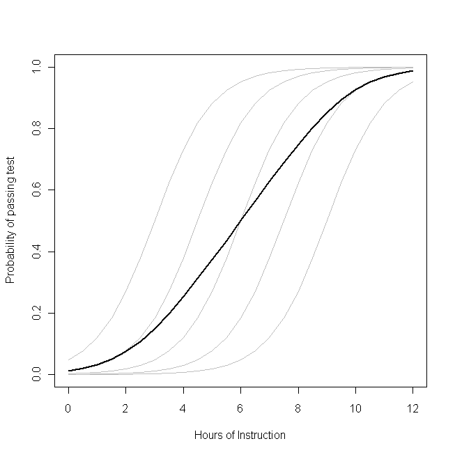
Imagine that this plot represents the underlying data generating process for the probability that a small class of students will be able to pass a test on some subject with a given number of hours of instruction on that topic. Each of the grey curves represents the probability of passing the test with varying amounts of instruction for one of the students. The bold curve is the average over the whole class. In this case, the effect of an additional hour of teaching conditional on the student’s attributes is β1_1–the same for each student (that is, there is not a random slope). Note, though, that the students baseline ability differs amongst them–probably due to differences in things like IQ (that is, there is a random intercept). The average probability for the class as a whole, however, follows a different profile than the students. The strikingly counter-intuitive result is this: an additional hour of instruction can have a sizable effect on the probability of each student passing the test, but have relatively little effect on the probable total proportion of students who pass. This is because some students might already have had a large chance of passing while others might still have little chance.
The question of whether you should use a GLMM or the GEE is the question of which of these functions you want to estimate. If you wanted to know about the probability of a given student passing (if, say, you were the student, or the student’s parent), you want to use a GLMM. On the other hand, if you want to know about the effect on the population (if, for example, you were the teacher, or the principal), you would want to use the GEE.
What are the best methods for checking a generalized linear mixed model (GLMM) for proper fit? Unfortunately, it isn’t as straightforward as it is for a general linear model. n linear models the requirements are easy to outline: linear in the parameters, normally distributed and independent residuals, and homogeneity of variance (that is, similar variance at all values of all predictors).
For linear models, there are well-described and well-implemented methods for checking each of these, both visual/descriptive methods and statistical tests.
It is not nearly as easy for GLMMs.
Assumption: Random effects come from a normal distribution
Let’s start with one of the more familiar elements of GLMMs, which is related to the random effects. There is an assumption that random effects—both intercepts and slopes—are normally distributed.
These are relatively easy to export to a data set in most statistical software (including SAS and R). Personally, I much prefer visual methods of checking for normal distributions, and typically go right to making histograms or normal probability plots (Q-Q plots) of each of the random effects.
If the histograms look roughly bell-shaped and symmetric, or the Q-Q plots generally fall close to a diagonal line, I usually consider this to be good enough.
If the random effects are not reasonably normally distributed, however, there are not simple remedies. In a general linear model outcomes can be transformed. In GLMMs they cannot.
Research is currently being conducted on the consequences of mis-specifying the distribution of random effects in GLMMs. (Outliers, of course, can be handled the same way as in generalized linear models—except that an entire random subject, as opposed to a single observation, may be examined.)
Assumption: The chosen link function is appropriate
Additional assumptions of GLMMs are more related to the generalized linear model side. One of these is the relationship of the numeric predictors to the parameter of interest, which is determined by the link function.
For both generalized linear models and GLMMs, it is important to understand that the most typical link functions (e.g., the logit for binomial data, the log for Poisson data) are not guaranteed to be a good representation of the relationship of the predictors with the outcomes.
Checking this assumption can become quite complicated as models become more crowded with fixed and random effects.
One relatively simple (though not perfect) way to approach this is to compare the predicted values to the actual outcomes.
With most GLMMs, it is best to compare averages of outcomes to predicted values. For example, with binomial models, one could take all of the values with predicted values near 0.5, 0.15, 0.25, etc., and average the actual outcomes (the 0s and 1s). You can then plot these average values against the predicted values.
If the general form of the model is correct, the differences between the predicted values and the averaged actual values will be small. (Of course how small depends on the number of observations and variance function).
No “patterns” in these differences should be obvious.
This is similar to the idea of the Hosmer-Lemeshow test for logistic regression models. If you suspect that the form of the link function is not correct, there are remedies. Possibilites include changing the link function, transforming numeric predictors, or (if necessary) categorizing continuous predictors.
Assumption: Appropriate estimation of variance
Finally, it is important to check the variability of the outcomes. This is also not as easy as it is for linear models, since the variance is not constant and is a function of the parameter being estimated.
Fortunately, this is one of the easier assumptions to check. One of the fit statistics your statistical software produces is a generalized chi-square that compares the magnitude of the model residuals to the theoretical variance.
The chi-square divided by its degrees of freedom should be approximately 1. If this statistic is too large, then the variance is “overdispersed” (larger than it should be). Alternatively, if the statistic is too small, the variance is “underdispersed.”
While the best way to approach this varies by distribution, there are options to adjust models for overdispersion that result in more conservative p-values.
9.5 Logit
Possible Analysis methods:
Below is a list of some analysis methods you may have encountered. Some of the methods listed are quite reasonable while others have either fallen out of favor or have limitations.
- Logistic regression, the focus of this page
- Probit regression. Probit analysis will produce results similar logistic regression. The choice of probit versus logit depends largely on individual preferences.
- OLS regression. When used with a binary response variable, this model is known as a linear probability model and can be used as a way to describe conditional probabilities. However, the errors (i.e., residuals) from the linear probability model violate the homoskedasticity and normality of errors assumptions of OLS regression, resulting in invalid standard errors and hypothesis tests. For a more thorough discussion of these and other problems with the linear probability model.
- Two-group discriminant function analysis. A multivariate method for dichotomous outcome variables.
- Hotelling’s T2. The 0/1 outcome is turned into the grouping variable, and the former predictors are turned into outcome variables. This will produce an overall test of significance but will not give individual coefficients for each variable, and it is unclear the extent to which each “predictor” is adjusted for the impact of the other “predictors.”
9.5.1 Odd’s Ratio
If you want to interpret the estimated effects as relative odds ratios,
just do exp(coef(x)) (gives you \(e^β\),
the multiplicative change in the odds ratio for \(y=1\)
if the covariate associated with \(β\) increases by 1).
For profile likelihood intervals for this quantity, you can do
require(MASS)
exp(cbind(coef(x), confint(x)))
To get the odds ratio, we need the classification cross-table of the original dichotomous DV and the predicted classification according to some probability threshold that needs to be chosen first.